Difference between revisions of "Overview of the Generic PCM"
(→Our team of developers) |
|||
| Line 24: | Line 24: | ||
TO BE MODIFIED (AND COMPLETED) by Aymeric | TO BE MODIFIED (AND COMPLETED) by Aymeric | ||
| + | |||
| + | == What is a GCM (alternative version by JL) == | ||
| + | |||
| + | A Global Climate Model (GCM) like the Generic PCM calculates the temporal evolution of the different variables (temperature, pressure, mass, mixing ratio of tracers/gas/clouds, winds, etc.) that control or describe the planetary meteorology and climate at different points of a 3D “grid” that covers the entire atmosphere. | ||
| + | |||
| + | To do that, the model solves 3D hydrodynamic equations that describe how atmospheric winds are created by various physical forcings (radiative heating/cooling, etc.) and how these winds transport and redistribute the various atmospheric fields (temperature, tracers, etc.). However, it can be shown that to a good level of approximation, the various forcings can be computed using only local conditions in a column of atmosphere, whereas long-range couplings between various points of the planet are mediated through atmospheric transport. | ||
| + | |||
| + | For these reasons, the 3D model is split in two components: | ||
| + | |||
| + | * '''a 3D dynamical core''' abble to integrate in time the general equations for atmospheric circulation when the various local forcings are known. This component (including source code) is common to all terrestrial-type atmospheres, and applicable in certain cases to the upper atmospheres of gas giant planets. | ||
| + | * '''a physical package''' that is specific to the planet in question (as it takes into account dedicated parametrizations representative of ongoing physical processes) and which computes atmospheric processes in each atmospheric column (which are sub-grid-scale from the point of view of the dynamical core). | ||
| + | |||
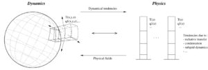
| + | [[File:Didi-eps-converted-to-1.png|thumb|Physics / Dynamics interface]] | ||
| + | |||
| + | In practice, we have several '''dynamical cores''' available with the model: LMDZ (global longitude/latitude grid), DYNAMICO (icosaedric grid), and WRF (rectangular box for local/regional studies) | ||
| + | |||
| + | From an initial state, the model calculates the temporal evolution of these variables, one timestep after another: | ||
| + | * At instant t, variables X<sub>t</sub> (temperature for example) are known at every grid point of the atmosphere. | ||
| + | * The physical model calculates the local time derivatives of the various variables -- called the tendencies -- ((δX/δt)<sub>1</sub>, (δX/δt)<sub>2</sub>, etc.) due to each physical phenomenon: for example, heating due to absorption of solar radiation and infrared cooling, mixing due to turbulence in the planetary boundary layer, condensation/evaporation of water vapor, etc. These tendencies are calculated via parameterization of the processes involved that try to capture the physical behavior of the atmopshere at the subgrid scale. | ||
| + | * These tendencies are passed to the dynamical core that integrates the model forward in time to the next time step, t + δt, by solving the hydrodynamical equations. | ||
| + | * This new state can be used to recompute the tendencies for the next time step and so on. | ||
| + | |||
| + | == Philosophy of the Generic PCM == | ||
| + | |||
| + | The accuracy and predictive power of any GCM is often dictated by the choice made for the physical phenomena that are included and for the way they are parametrized. To be accurate, many Earth-centric climate models use very complex parametrization that are heavily tuned on Earth observations. Such parametrization can, however, behave very poorly far from the parameter space where they have been validated, thus reducing their predictive power for exotic atmospheres. | ||
| + | |||
| + | As the goal of the Generic PCM is to model the climate of very different planets with the same model, a particular emphasis has been put on using simple parametrizations based as much as possible on ab-initio physical equations and conservation principles to avoid unphysical behaviors in extreme regimes. | ||
| + | |||
== GCM inputs and outputs == | == GCM inputs and outputs == | ||
Revision as of 17:39, 31 August 2022
Contents
What is a GCM?
Our Global Climate Model (GCM) calculates the temporal evolution of the different variables (temperature, pressure, mass, mixing ratio of tracers/gas/clouds, winds, etc.) that control or describe the planetary meteorology and climate at different points of a 3D “grid” that covers the entire atmosphere.
From an initial state, the model calculates the temporal evolution of these variables, one timestep after another:
- At instant t, variables Xt (temperature for example) are known at every grid point of the atmosphere.
- We calculate the evolution (the tendencies) (δX/δt)1, (δX/δt)2, etc.) due to each physical phenomenon, calculated via the parameterization thereof (e.g., heating due to absorption of solar radiation, mixing due to turbulence in the planetary boundary layer, etc.).
- In order to move on to the next time step, t + δt, we can calculate Xt+δt from Xt and (δX/δt). This is formally known as the time integration of the variables. (For example, Xt+δt = Xt + (δX/δt)1δt + (δX/δt)2δt + ...)
The main task of the model is to calculate these tendencies (δX/δt) arising from the different parameterized phenomena.
TO BE MODIFIED (AND COMPLETED) by Jeremy
Physical vs dynamical core
In practice, the 3D model is split in two components:
- a dynamical core containing the numerical solution of the general equations for atmospheric circulation. This component (including source code) is common to all terrestrial-type atmospheres, and applicable in certain cases to the upper atmospheres of gas giant planets.
- a physical package that is specific to the planet in question (as it takes into account dedicated parametrizations representative of ongoing physical processes) and which computes atmospheric processes in each atmospheric column (which are sub-grid-scale from the point of view of the dynamical core).
In practice, we do have several dynamical cores available with the model: LMDZ (global longitude/latitude grid), DYNAMICO (icosaedric grid) and WRF (rectangular box for local/regional studies)
TO BE MODIFIED (AND COMPLETED) by Aymeric
What is a GCM (alternative version by JL)
A Global Climate Model (GCM) like the Generic PCM calculates the temporal evolution of the different variables (temperature, pressure, mass, mixing ratio of tracers/gas/clouds, winds, etc.) that control or describe the planetary meteorology and climate at different points of a 3D “grid” that covers the entire atmosphere.
To do that, the model solves 3D hydrodynamic equations that describe how atmospheric winds are created by various physical forcings (radiative heating/cooling, etc.) and how these winds transport and redistribute the various atmospheric fields (temperature, tracers, etc.). However, it can be shown that to a good level of approximation, the various forcings can be computed using only local conditions in a column of atmosphere, whereas long-range couplings between various points of the planet are mediated through atmospheric transport.
For these reasons, the 3D model is split in two components:
- a 3D dynamical core abble to integrate in time the general equations for atmospheric circulation when the various local forcings are known. This component (including source code) is common to all terrestrial-type atmospheres, and applicable in certain cases to the upper atmospheres of gas giant planets.
- a physical package that is specific to the planet in question (as it takes into account dedicated parametrizations representative of ongoing physical processes) and which computes atmospheric processes in each atmospheric column (which are sub-grid-scale from the point of view of the dynamical core).
In practice, we have several dynamical cores available with the model: LMDZ (global longitude/latitude grid), DYNAMICO (icosaedric grid), and WRF (rectangular box for local/regional studies)
From an initial state, the model calculates the temporal evolution of these variables, one timestep after another:
- At instant t, variables Xt (temperature for example) are known at every grid point of the atmosphere.
- The physical model calculates the local time derivatives of the various variables -- called the tendencies -- ((δX/δt)1, (δX/δt)2, etc.) due to each physical phenomenon: for example, heating due to absorption of solar radiation and infrared cooling, mixing due to turbulence in the planetary boundary layer, condensation/evaporation of water vapor, etc. These tendencies are calculated via parameterization of the processes involved that try to capture the physical behavior of the atmopshere at the subgrid scale.
- These tendencies are passed to the dynamical core that integrates the model forward in time to the next time step, t + δt, by solving the hydrodynamical equations.
- This new state can be used to recompute the tendencies for the next time step and so on.
Philosophy of the Generic PCM
The accuracy and predictive power of any GCM is often dictated by the choice made for the physical phenomena that are included and for the way they are parametrized. To be accurate, many Earth-centric climate models use very complex parametrization that are heavily tuned on Earth observations. Such parametrization can, however, behave very poorly far from the parameter space where they have been validated, thus reducing their predictive power for exotic atmospheres.
As the goal of the Generic PCM is to model the climate of very different planets with the same model, a particular emphasis has been put on using simple parametrizations based as much as possible on ab-initio physical equations and conservation principles to avoid unphysical behaviors in extreme regimes.
GCM inputs and outputs
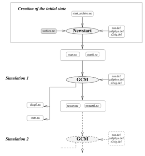
The input files are the files needed to initialize the model (state of the atmosphere at instant t0 as well as a dataset of boundary conditions). The output files are “historical files”, archives of the atmospheric flow history as simulated by the model, the “diagfi files”, the “stats files”, the daily averages, and so on.
TO BE COMPLETED
start and startfi files
TO BE COMPLETED
start vs restart files
TO BE COMPLETED
.def files
List of needed .def files:
- callphys.def: Physical parameters
- run.def: Numerical parameters
- gases.def: List of gases
- traceur.def: Numerical traceurs in the atmosphere
- z2sig.def: Pseudo-altitudes (in km) at which the user wants to set the vertical levels
- diagfi.def (optionnal): List of wanted outputs
input data
TO BE COMPLETED
output files
diagfi.nc diagspec_IR.nc / diagspec_VI.nc stats.nc etc.
TO BE COMPLETED
Our team of developers
TO BE COMPLETED

