Other GCM Configurations worth knowing about
Contents
3D lon-lat LMDZ setup
early Mars
It is already described in the Quick Install and Run section.
== Earth with slab ocean ==rcm1d
TBD by Siddharth, once all changes have been committed (also need a validation of the model on Earth to be sure)
TRAPPIST-1e with photochemistry
A temperate rocky planet in synchronous rotation around a low mass star.
Here is an example to simulate the planet TRAPPIST-1e with an Earth atmosphere using the photochemical module of the GCM.
To install the model and run it, follow Quick Install and Run but with the following changes:
GCM Input Datafiles and Datasets
Section GCM Input Datafiles and Datasets download the TRAPPIST-1e files (instead of the early Mars files):
wget -nv --no-check-certificate https://web.lmd.jussieu.fr/~lmdz/planets/generic/reference_setups/bench_trappist1e_photochemistry_64x48x30_b38x36.tar.gz
You can find the same type of file with the additional folder containing the chemical network file:
callphys.def  gases.def  startfi.nc  traceur.def
datadir/      run.def    start.nc    z2sig.def
chemnetwork/
Compiling the GCM
Prior to a first compilation: setting up the target architecture files
The chemical solver require the libraries BLAS and LAPACK which need to be specified in the arch*.fcm file:
%COMPILER            gfortran
%LINK                gfortran
%AR                  ar
%MAKE                make
%FPP_FLAGS           -P -traditional
%FPP_DEF             NC_DOUBLE LAPACK BLAS SGEMV=DGEMV SGEMM=DGEMM
%BASE_FFLAGS         -c -fdefault-real-8 -fdefault-double-8 -ffree-line-length-none -fno-align-commons
%PROD_FFLAGS         -O3
%DEV_FFLAGS          -O
%DEBUG_FFLAGS        -ffpe-trap=invalid,zero,overflow -fbounds-check -g3 -O0 -fstack-protector-all -finit-real=snan -fbacktrace
%MPI_FFLAGS
%OMP_FFLAGS
%BASE_LD             -llapack -lblas
%MPI_LD
%OMP_LD
Specific to photochemistry: set hard coded reactions
In /LMDZ.GENERIC/libf/aeronogeneric/chimiedata_h.F90 you can hard code reaction if needed, for instance because the reaction rate is very specific and out of the generic formula or your photochemical reaction does not use a regular cross section.
The TRAPPIST-1e test case use 3 hard coded reactions.
- Uncomment the following lines to fill reaction species indexes:
!===========================================================
!      r001 : HNO3 + rain -> H2O
!===========================================================
nb_phot = nb_phot + 1
indice_phot(nb_phot) = z3spec(1.0, indexchim('hno3'), 1.0, indexchim('h2o_vap'), 0.0, 1)

!===========================================================
!      e001 : CO + OH -> CO2 + H
!===========================================================
nb_reaction_4 = nb_reaction_4 + 1
indice_4(nb_reaction_4) = z4spec(1.0, indexchim('co'), 1.0, indexchim('oh'), 1.0, indexchim('co2'), 1.0, indexchim('h'))

!ccccccccccccccccccccccccccccccccccccccccccccccccccccccccccccccccccc
!     photodissociation of NO : NO + hv -> N + O
!ccccccccccccccccccccccccccccccccccccccccccccccccccccccccccccccccccc
nb_phot = nb_phot + 1
indice_phot(nb_phot) = z3spec(1.0, indexchim('no'), 1.0, indexchim('n'), 1.0, indexchim('o'))
- Uncomment the following lines to fill reaction rates:
!----------------------------------------------------------------------
!     carbon reactions
!----------------------------------------------------------------------

!---  e001: oh + co -> co2 + h

      nb_reaction_4 = nb_reaction_4 + 1

!     joshi et al., 2006

      do ilev = 1,nlayer
         k1a0 = 1.34*2.5*dens(ilev)                                  &
               *1/(1/(3.62e-26*t(ilev)**(-2.739)*exp(-20./t(ilev)))  &
               + 1/(6.48e-33*t(ilev)**(0.14)*exp(-57./t(ilev))))     ! typo in paper corrected
         k1b0 = 1.17e-19*t(ilev)**(2.053)*exp(139./t(ilev))          &
              + 9.56e-12*t(ilev)**(-0.664)*exp(-167./t(ilev))
         k1ainf = 1.52e-17*t(ilev)**(1.858)*exp(28.8/t(ilev))        &
                + 4.78e-8*t(ilev)**(-1.851)*exp(-318./t(ilev))
         x = k1a0/(k1ainf - k1b0)
         y = k1b0/(k1ainf - k1b0)
         fc = 0.628*exp(-1223./t(ilev)) + (1. - 0.628)*exp(-39./t(ilev))  &
            + exp(-t(ilev)/255.)
         fx = fc**(1./(1. + (alog(x))**2))                           ! typo in paper corrected
         k1a = k1a0*((1. + y)/(1. + x))*fx
         k1b = k1b0*(1./(1.+x))*fx

         v_4(ilev,nb_reaction_4) = k1a + k1b
      end do

!----------------------------------------------------------------------
!     washout r001 : HNO3 + rain -> H2O
!----------------------------------------------------------------------

nb_phot = nb_phot + 1

rain_h2o  = 100.e-6
!rain_rate = 1.e-6  ! 10 days
rain_rate = 1.e-8

do ilev = 1,nlayer
   if (c(ilev,indexchim('h2o_vap'))/dens(ilev) >= rain_h2o) then
      v_phot(ilev,nb_phot) = rain_rate
   else
      v_phot(ilev,nb_phot) = 0.
   end if
end do

!ccccccccccccccccccccccccccccccccccccccccccccccccccccccccccccccccccc
!     photodissociation of NO
!ccccccccccccccccccccccccccccccccccccccccccccccccccccccccccccccccccc

nb_phot = nb_phot + 1

colo3(nlayer) = 0.
!     ozone columns for other levels (molecule.cm-2)
do ilev = nlayer-1,1,-1
   colo3(ilev) = colo3(ilev+1) + (c(ilev+1,indexchim('o3')) + c(ilev,indexchim('o3')))*0.5*avocado*1e-4*((press(ilev) - press(ilev+1))*100.)/(1.e-3*zmmean(ilev)*g*dens(ilev))
end do
call jno(nlayer, c(nlayer:1:-1,indexchim('no')), c(nlayer:1:-1,indexchim('o2')), colo3(nlayer:1:-1), dens(nlayer:1:-1), press(nlayer:1:-1), sza, v_phot(nlayer:1:-1,nb_phot))
- Change the following lines to set the number of hard coded reactions:
integer, parameter :: nphot_hard_coding = 2
integer, parameter :: n4_hard_coding    = 1
integer, parameter :: n3_hard_coding    = 0
Compiling a test case (TRAPPIST-1e)
Change the following compiling option:
-d 64x48x30 -b 38x36
NB: option -b is mandatory to change while option -d will still run with lower or higher resolution (if z2sig.def remains coherent with the number of altitude levels, meaning at least as many altitude levels defined as the number of levels wanted).
TRAPPIST-1c in Venus-like conditions
A warm rocky planet in synchronous rotation around a low mass star. Here we provide an example to simulate the atmosphere of Trappist-1c, assuming it evolved to a modern Venus-like atmosphere.
The planetary parameters are taken from Algol et al. 2021 and can be found in this table Media:Planetary_parameters_Trappist1c.png
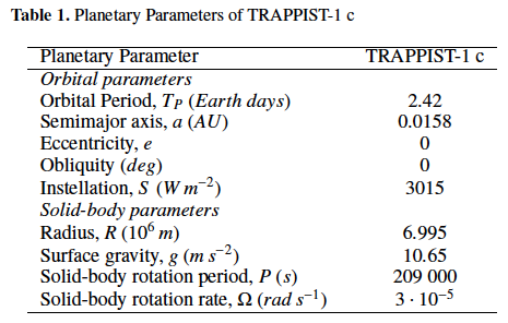
First, install the model and run it, following Quick Install and Run but instead of Early Mars files, please download bench_trappist1c_64x48x50_b32x36 using this command:
wget -nv --no-check-certificate https://web.lmd.jussieu.fr/~lmdz/planets/generic/reference_setups/bench_trappist1c_64x48x50_b32x36.tar.gz
Compiling a test case (TRAPPIST-1c)
Change the following compiling option:
-d 64x48x50 -b 32x36
You can find the same type of ASCII *def files than in the case of Early Mars, but adapted to the planet's characteristics and orbital parameters of Trappist 1c.
In particular callphys.def contains the following changes:
- The planet is assumed to be in 1:1 spin-orbit resonance, therefore
  diurnal = .false.
  tlocked = .true.
- The planet equilibrium temperature is about 342 K
tplanet = 341.9
- The host star is TRAPPIST1, with a stellar flux at 1 AU of 0.7527 [W m-2]
  stelspec_file = spectrum_TRAPPIST1_2022.dat
  tstellar = 2600.
  Fat1AU = 0.7527
- Fixed aerosol distribution, no radiative active tracers (no evaporation/condensation of H2O and CO2):
  aerofixed     = .true.
  aeroco2       = .false.
  aeroh2o       = .false.
- No water cycle model, no water cloud formation or water precipitation, no CO2 condensation:
  water         = .false.
  watercond     = .false.
  waterrain     = .false.
  hydrology     = .false.
  nonideal      = .true.
  co2cond       = .false.
- Following Haus et al. 2015 a prescribed radiatively active cloud model is included.
It can be activated/deactivated with the flag aerovenus.
aerovenus = .true.
- Mode 1, 2, 2p, 3 and the "unknown" UV absorber can be included/excluded by setting to true/false the following keywords. The characteristics of each mode (e.g. effect radius, effective variance) are based on Venus Express/ESA observations and can be found in this table Media:Table1 aerosolVenus trappist1c.png
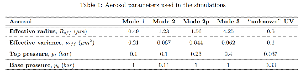
  aerovenus1    = .true.
  aerovenus2    = .true.
  aerovenus2p   = .true.
  aerovenus3    = .true.
  aerovenusUV   = .true.
The cloud model is prescribed from 1 to 0.037 bar pressure layers. For each mode, the top/bottom pressure can be modified by hard-coding model routine aerosol_opacity.F90. Here below an example for mode 1 particles, where the top pressure layer and bottom pressure layer are prescribed at 0.1 bar and 1 bar, respectively:
!       1. Initialization
          aerosol(1:ngrid,1:nlayer,iaer)=0.0
          p_bot = 1.e5 ! bottom pressure [Pa]
          p_top = 1.e4
          h_bot = 1.0e3 ! bottom scale height [m]
          h_top = 5.0e3
TO BE COMPLETED BY GABRIELLA
mini-Neptune GJ1214b
A warm mini-Neptune
TO BE COMPLETED BY BENJAMIN
3D DYNAMICO setup
Due to the rich dynamical activities in their atmospheres (banded zonal jets, eddies, vortices, storms, equatorial oscillations,...) resulting from multi-scale dynamic interactions, the Global Climate Modelling of the giant planet requires to resolve eddies arising from hydrodynamical instabilities to correctly establish the planetary-scaled jets regime. To this purpose, their Rossby radius deformation $$L_D$$, which is the length scale at which rotational effects become as important as buoyancy or gravity wave effects in the evolution of the flow about some disturbance, is calculated to determine the most suitable horizontal grid resolution. At mid-latitude range, for the giant planets, $$L_D$$ is of the same order of magnitude as that of the Earth. As the giant planets have a size of roughly 10 times the Earth size (i.e., Jupiter and Saturn), the modelling grid must be of a horizontal resolution of 0.5$$^{\circ}$$ over longitude and latitude (vs 5$$^{\circ}$$ for the Earth), considering 3 grid points to resolved $$L_D$$. Moreover, to have a chance to model the equatorial oscillation, meridional cell circulations and/or a seasonal inter-hemispheric circulation, a giant planet GCM must also include a high vertical resolution. Indeed, these climate phenomena have been studied for decades for the Earth's atmosphere, and result from small- and large-scale interactions between the troposphere and stratosphere. This implies that the propagation of dynamic instabilities, waves and turbulence should be resolved as far as possible along the vertical. Contrary to horizontal resolution, it doesn't really exist a criterion (similar to $$L_D$$) to determine the most suitable vertical grid resolution and still an adjustable parameter according to the processes to be represented. However, we advise the user to set a vertical resolution of at least 5 grid points per scale height as first stage. Finally, these atmospheres are cold, with long radiative response time which needs radiative transfer computations over decade-long years of Jupiter (given that a Jupiter year $$\approx$$ 12 Earth years), Saturn ( a Saturn year $$\approx$$ 30 Earth years), Uranus (a Uranus year $$\approx$$ 84 earth years) or Neptune (a Neptune year $$\approx$$ 169 Earth years), depending on the chosen planet.
To be able to deal with these three -- and non-exhaustive -- requirements to build a giant planet GCM, we need massive computational ressources. For this, we use a dynamical core suitable and numerically stable for massive parallel ressource computations: DYNAMICO [Dubos et al,. 2015].
In these two following subsections, we purpose an example of installation for Jupiter and a Hot Jupiter. All the install, compiling, setting and parameters files for each giant planets could be found on: https://gitlab.in2p3.fr/aymeric.spiga/dynamico-giant (the old repo is archived as read-only https://github.com/aymeric-spiga/dynamico-giant)
The DYNAMICO-giant wiki is here
If you have already downloaded LMDZ.COMMON, LMDZ.GENERIC, IOIPSL, ARCH, you only have to download:
ICOSAGCM: the DYNAMICO dynamical core
git clone https://gitlab.in2p3.fr/ipsl/projets/dynamico/dynamico.git ICOSAGCM
cd ICOSAGCM
git checkout 110016896ae9e85e614af43223b18fe38f211020   # Version du 6 nov. 2024
ICOSA_LMDZ: the interface using to link LMDZ.GENERIC physical packages and ICOSAGCM
svn update -r 3729 -q ICOSA_LMDZ # Version du 18 avr. 2025
XIOS (XML Input Output Server): the library to interpolate input/output fields between the icosahedral and longitude/latitude regular grids on fly
svn co -r 2626 -q http://forge.ipsl.jussieu.fr/ioserver/svn/XIOS/trunk XIOS # Version du 22 mar. 2024
If you haven't already download LMDZ.COMMON, LMDZ.GENERIC, IOIPSL, ARCH, you can use the install.sh script provided by the GitLab repository.
Once each part of the GCM is downloaded, you are able to compile it.
Firstly, you have to define your target architecture file (hereafter named YOUR_ARCH_FILE) where you will fill in all the necessary information about the local environment, where libraries are located, which compiler, and compiler options will be used, etc.
Some architecture files related to specific machines are provided in the ARCH directory, which are referenced in the following lines without the prefix 'arch-' (i.e., arch-X64_IRENE-AMD.env will be referenced as X64_IRENE-AMD).
The main specificity of DYNAMICO-giant is that every main parts of the model (ICOSAGCM, LMDZ.COMMON and LMDZ.GENERIC) are compiled as libraries, and settings and running configuration are managed by the ICOSA_LMDZ interface.
First, you have to compile IOIPSL,
cd LMDZ.COMMON/ioipsl/
    ./install_ioipsl_YOUR-MACHINE.bash
cd ../../
then XIOS library,
cd XIOS/
    ./make_xios --prod --arch YOUR_ARCH_FILE --arch_path ../ARCH --job 8 --full
cd -
the physics packaging,
cd LMDZ.COMMON/
    ./makelmdz_fcm -p generic -p_opt "-b 20x25" -prod -parallel mpi -libphy -io xios -arch YOUR_ARCH_FILE -arch_path ../ARCH -j 8 -full
cd -
the dynamical core DYNAMICO (located in ICOSAGCM directory, named from the icosahedral shape of the horizontal mesh),
cd ICOSAGCM/
    ./make_icosa -prod -parallel mpi -external_ioipsl -with_xios -arch YOUR_ARCH_FILE -arch_path ../ARCH -job 8 -full
cd -
and finally the ICOSA_LMDZ interface
cd ICOSA_LMDZ/
    ./make_icosa_lmdz -p generic -p_opt "-b 20x25" -parallel mpi -arch YOUR_ARCH_FILE -arch_path ../ARCH -job 8 -nodeps
This last step is a bit redundant with the two previous one, hence make_icosa_lmdz will execute ./make_icosa (in the ICOSAGCM directory) and ./makelmdz_fcm (in the LMDZ.COMMON directory) to create and source the architecture files shared between all parts of the model, as well as create the intermediate file config.fcm. As you have already compiled these two elements, make_icosa_lmdz should only create the linked architecture files, config.fcm and compile the interface. Here, -nodeps option prevents the checking of XIOS and IOIPSL compilation, which saves you from recompiling these two elements again.
Finally, your executable programs should appeared in ICOSA_LMDZ/bin subdirectory, as icosa_lmdz.exe and in XIOS/bin subdirectory, as xios_server.exe
All these compiling steps are summed up in make_isoca_lmdz program that should be adapted to your own computational settings (i.e., through you target architecture file).
./make_icosa_lmdz -p generic -p_opt "-b 20x25" -parallel mpi -arch YOUR_ARCH_FILE -arch_path ../ARCH -job 8 -full
Here, -full option assure the compilation of each part (IOIPSL, XIOS, LMDZ.COMMON, ICOSAGCM and ICOSA_LMDZ) of the model.
Now you can move your two executable files to your working directory and start to run your own simulation of Jupiter or a Hot Jupiter, as what follows.
Note: If you are using the GitLab file architecture (https://gitlab.in2p3.fr/aymeric.spiga/dynamico-giant), you should be able to compile the model directly from your working directory (for instance dynamico-giant/jupiter/) by using the compile_occigen.sh program, which has to be adapted to your machine/cluster.
Note 2 : Depending on the compiler module you use, especially with gfortran, you may need to modify the tracers_icosa.F90 file located in the src directory in order to successfully compile ICOSAGCM. For example, if you are using GCC/11.3.0 and OpenMPI/4.1.4, you must update the insert_tracer_output subroutine as follows:
SUBROUTINE insert_tracer_output
      USE xios_mod
      USE grid_param
      IMPLICIT NONE
      TYPE(xios_fieldgroup) :: fieldgroup_hdl
      TYPE(xios_field) :: field_hdl
      INTEGER :: iq
      CHARACTER(len=1000) :: tracername1
      CHARACTER(len=1000) :: tracername2
      CHARACTER(len=1000) :: tracername3

      CALL xios_get_handle("standard_output_tracers", fieldgroup_hdl)
      DO iq = 1, nqtot
         tracername1 = "tracer_"//TRIM(tracers(iq)%name)
         CALL xios_add_child(fieldgroup_hdl, field_hdl, tracername1)
         CALL xios_set_attr(field_hdl, name=TRIM(tracers(iq)%name))
      END DO

      CALL xios_get_handle("standard_output_tracers_init", fieldgroup_hdl)
      DO iq = 1, nqtot
         tracername2 = "tracer_"//TRIM(tracers(iq)%name)//"_init"
         tracername3 = TRIM(tracers(iq)%name)//"_init"
         CALL xios_add_child(fieldgroup_hdl, field_hdl, tracername2)
         CALL xios_set_attr(field_hdl, name=tracername3)
      END DO

   END SUBROUTINE insert_tracer_output
Jupiter with DYNAMICO
Using a new dynamical core implies new setting files, in addition or as a replacement of those relevant to LMDZ.COMMON dynamical core using.
There are two kind of setting files:
A first group relevant to DYNAMICO:
- context_dynamico.xml: Configuration file for DYNAMICO for reading and writing files using XIOS, mainly used when you want to check the installation of ICOSAGCM with an Held and Suarez test case. When your installation, compilation and run environment is fully functional, the dynamic core output files will not (necessarily) be useful and you can disable their writing.
- file_def_dynamico.xml: Definition of output diagnostic files which will be written into the output files only related to ICOSAGCM.
- field_def_dynamico.xml: Definition of all existing variables that can be output from DYNAMICO.
- tracer.def: Definition of the name and physico-chemical properties of the tracers which will be advected by the dynamical core. For now, there is two files related to tracers, we are working to harmonise it.
A second group relevant to LMDZ.GENERIC physical packages:
- context_lmdz_physics.xml: File in which are defined the horizontal grid, vertical coordinate, output file(s) definition, with the setting of frequency output writing, time unit, geophysical variables to be written, etc. Each new geophysical variables added here have to be defined in the field_def_physics.xml file.
- field_def_physics.xml: Definition of all existing variables that can be output from the physical packages interfaced with DYNAMICO. This is where you will add each geophysical fields that you want to appear in the Xhistins.nc output files. For instance, related to the thermal plume scheme using for Jupiter's tropospheric dynamics, we have added the following variables:
 1              <field id="h2o_vap"
 2                    long_name="Vapor mass mixing ratio"
 3                    unit="kg/kg" />
 4             <field id="h2o_ice"
 5                    long_name="Vapor mass mixing ratio"
 6                    unit="kg/kg" />
 7             <field id="detr"
 8                    long_name="Detrainment"
 9                    unit="kg/m2/s" />
10             <field id="entr"
11                    long_name="Entrainment"
12                    unit="kg/m2/s" />
13             <field id="w_plm"
14                    long_name="Plume vertical velocity"
15                    unit="m/s" />
- callphys.def: This setting file is used either with DYNAMICO or LMDZ.COMMON and allows the user to choose the physical parametrisation schemes and their appropriate main parameter values relevant to the planet being simulated. In our case of Jupiter, there are some specific parametrisations that should be added or modified from the example given as link at the beginning of this line:
  1 # Diurnal cycle ?  if diurnal=false, diurnally averaged solar heating
  2 diurnal      = .false. #.true.
  3 # Seasonal cycle ? if season=false, Ls stays constant, to value set in "start"
  4 season       = .true.
  5 # Tidally resonant orbit ? must have diurnal=false, correct rotation rate in newstart
  6 tlocked      = .false.
  7 # Tidal resonance ratio ? ratio T_orbit to T_rotation
  8 nres         = 1
  9 # Planet with rings?
 10 rings_shadow = .false.
 11 # Compute latitude-dependent gravity field??
 12 oblate       = .true.
 13 # Include non-zero flattening (a-b)/a?
 14 flatten      = 0.06487
 15 # Needed if oblate=.true.: J2
 16 J2           = 0.01470
 17 # Needed if oblate=.true.: Planet mean radius (m)
 18 Rmean        = 69911000.
 19 # Needed if oblate=.true.: Mass of the planet (*1e24 kg)
 20 MassPlanet   = 1898.3
 21 # use (read/write) a startfi.nc file? (default=.true.)
 22 startphy_file = .false.
 23 # constant value for surface albedo (if startphy_file = .false.)
 24 surfalbedo   = 0.0
 25 # constant value for surface emissivity (if startphy_file = .false.)
 26 surfemis     = 1.0
 27
 28 # the rad. transfer is computed every "iradia" physical timestep
 29 iradia           = 160
 30 # folder in which correlated-k data is stored ?
 31 corrkdir         = Jupiter_HITRAN2012_REY_ISO_NoKarko_T460K_article2019_gauss8p8_095
 32 # Uniform absorption coefficient in radiative transfer?
 33 graybody         = .false.
 34 # Characteristic planetary equilibrium (black body) temperature
 35 # This is used only in the aerosol radiative transfer setup. (see aerave.F)
 36 tplanet          = 100.
 37 # Output global radiative balance in file 'rad_bal.out' - slow for 1D!!
 38 meanOLR          = .false.
 39 # Variable gas species: Radiatively active ?
 40 varactive        = .false.
 41 # Computes atmospheric specific heat capacity and
 42 # could calculated by the dynamics, set in callphys.def or calculeted from gases.def.
 43 # You have to choose: 0 for dynamics (3d), 1 for forced in callfis (1d) or 2: computed from gases.def (1d)
 44 # Force_cpp and check_cpp_match are now deprecated.
 45 cpp_mugaz_mode = 0
 46 # Specific heat capacity in J K-1 kg-1 [only used if cpp_mugaz_mode = 1]
 47 cpp              = 11500.
 48 # Molecular mass in g mol-1 [only used if cpp_mugaz_mode = 1]
 49 mugaz            = 2.30
 50 ### DEBUG
 51 # To not call abort when temperature is outside boundaries:
 52 strictboundcorrk = .false.
 53 # To not stop run when temperature is greater than 400 K for H2-H2 CIA dataset:
 54 strictboundcia = .false.
 55 # Add temperature sponge effect after radiative transfer?
 56 callradsponge    = .false.
 57
 58 Fat1AU = 1366.0
 59
 60 ## Other physics options
 61 ## ~~~~~~~~~~~~~~~~~~~~~
 62 # call turbulent vertical diffusion ?
 63 calldifv    = .false.
 64 # use turbdiff instead of vdifc ?
 65 UseTurbDiff = .true.
 66 # call convective adjustment ?
 67 calladj     = .true.
 68 # call thermal plume model ?
 69 calltherm   = .true.
 70 # call thermal conduction in the soil ?
 71 callsoil    = .false.
 72 # Internal heat flux (matters only if callsoil=F)
 73 intheat     = 7.48
 74 # Remove lower boundary (e.g. for gas giant sims)
 75 nosurf      = .true.
 76 #########################################################################
 77 ## extra non-standard definitions for Earth
 78 #########################################################################
 79
 80 ## Thermal plume model options
 81 ## ~~~~~~~~~~~~~~~~~~~~~~~~~~~
 82 dvimpl               = .true.
 83 r_aspect_thermals    = 2.0
 84 tau_thermals         = 0.0
 85 betalpha             = 0.9
 86 afact                = 0.7
 87 fact_epsilon         = 2.e-4
 88 alpha_max            = 0.7
 89 fomass_max           = 0.5
 90 pres_limit           = 2.e5
 91
 92 ## Tracer and aerosol options
 93 ## ~~~~~~~~~~~~~~~~~~~~~~~~~~
 94 # Ammonia cloud (Saturn/Jupiter)?
 95 aeronh3             = .true.
 96 size_nh3_cloud      = 10.D-6
 97 pres_nh3_cloud      = 1.1D5                        # old: 9.D4
 98 tau_nh3_cloud       = 10.                          # old: 15.
 99 # Radiatively active aerosol (Saturn/Jupiter)?
100 aeroback2lay         = .true.
101 optprop_back2lay_vis = optprop_jupiter_vis_n20.dat
102 optprop_back2lay_ir  = optprop_jupiter_ir_n20.dat
103 obs_tau_col_tropo    = 4.0
104 size_tropo           = 5.e-7
105 pres_bottom_tropo    = 8.0D4
106 pres_top_tropo       = 1.8D4
107 obs_tau_col_strato   = 0.1D0
108 # Auroral aerosols (Saturn/Jupiter)?
109 aeroaurora         = .false.
110 size_aurora        = 3.e-7
111 obs_tau_col_aurora = 2.0
112
113 # Radiatively active CO2 aerosol?
114 aeroco2            = .false.
115 # Fixed CO2 aerosol distribution?
116 aerofixco2     = .false.
117 # Radiatively active water aerosol?
118 aeroh2o        = .false.
119 # Fixed water aerosol distribution?
120 aerofixh2o     = .false.
121 # basic dust opacity
122 dusttau        = 0.0
123 # Varying H2O cloud fraction?
124 CLFvarying     = .false.
125 # H2O cloud fraction if fixed?
126 CLFfixval      = 0.0
127 # fixed radii for cloud particles?
128 radfixed       = .false.
129 # number mixing ratio of CO2 ice particles
130 Nmix_co2       = 100000.
131 # number mixing ratio of water particles (for rafixed=.false.)
132 Nmix_h2o       = 1.e7
133 # number mixing ratio of water ice particles (for rafixed=.false.)
134 Nmix_h2o_ice   = 5.e5
135 # radius of H2O water particles (for rafixed=.true.):
136 rad_h2o        = 10.e-6
137 # radius of H2O ice particles (for rafixed=.true.):
138 rad_h2o_ice    = 35.e-6
139 # atm mass update due to tracer evaporation/condensation?
140 mass_redistrib = .false.
141
142 ## Water options
143 ## ~~~~~~~~~~~~~
144 # Model water cycle
145 water         = .true.
146 # Model water cloud formation
147 watercond     = .true.
148 # Model water precipitation (including coagulation etc.)
149 waterrain     = .true.
150 # Use simple precipitation scheme?
151 precip_scheme = 1
152 # Evaporate precipitation?
153 evap_prec     = .true.
154 # multiplicative constant in Boucher 95 precip scheme
155 Cboucher      = 1.
156 # Include hydrology ?
157 hydrology     = .false.
158 # H2O snow (and ice) albedo ?
159 albedosnow    = 0.6
160 # Maximum sea ice thickness ?
161 maxicethick   = 10.
162 # Freezing point of seawater (degrees C) ?
163 Tsaldiff      = 0.0
164 # Evolve surface water sources ?
165 sourceevol    = .false.
166
167 ## CO2 options
168 ## ~~~~~~~~~~~
169 # call CO2 condensation ?
170 co2cond       = .false.
171 # Set initial temperature profile to 1 K above CO2 condensation everywhere?
172 nearco2cond   = .false.
- gases.def: File containing the gas composition of the atmosphere you want to model, with their molar mixing ratios.
 1 # gases
 2 5
 3 H2_
 4 He_
 5 CH4
 6 C2H2
 7 C2H6
 8 0.863
 9 0.134
10 0.0018
11 1.e-7
12 1.e-5
13 # First line is number of gases
14 # Followed by gas names (always 3 characters)
15 # and then molar mixing ratios.
16 # mixing ratio -1 means the gas is variable.
- jupiter_const.def: Files that gather all orbital and physical parameters of Jupiter.
- traceur.def: At this time, only two tracers are used for modelling Jupiter atmosphere, so the traceur.def file is summed up as follow
1 2
2 h2o_vap
3 h2o_ice
Two additional files are used to set the running parameter of the simulation itself:
- run_icosa.def: file containing parameters for ICOSAGCM to execute the simulation, use to determine the horizontal and vertical resolutions, the number of processors, the number of subdivisions, the duration of the simulation, etc.
- run.def: file which brings together all the setting files and will be reading by the interface ICOSA_LMDZ to link each part of the model (ICOSAGCM, LMDZ.GENERIC) with its particular setting file(s) when the library XIOS does not take action (through the .xml files).
 1 ###########################################################################
 2 ### INCLUDE OTHER DEF FILES (physics, specific settings, etc...)
 3 ###########################################################################
 4 INCLUDEDEF=run_icosa.def
 5
 6 INCLUDEDEF=jupiter_const.def
 7
 8 INCLUDEDEF=callphys.def
 9
10
11 prt_level=0
12
13 ## iphysiq must be same as itau_physics
14 iphysiq=40
Hot Jupiter with DYNAMICO
Modelling the atmosphere of Hot Jupiter is challenging because of the extreme temperature conditions, and the fact that these planets are gas giants. Therefore, using a dynamical core such as Dynamico is strongly recommended. Here, we discuss how to perform a cloudless simulation of the Hot Jupiter WASP-43 b, using Dynamico.
1st step: You need to go to the github mentionned previously for Dynamico: https://github.com/aymeric-spiga/dynamico-giant. Git clone this repo on your favorite cluster, and checkout to the "hot_jupiter" branch.
2nd step: Now, run the install.sh script. This script will install all the required models (LMDZ.COMMON, LMDZ.GENERIC,ICOSA_LMDZ,XIOS,FCM,ICOSAGCM). At this point, you only miss IOIPSL. To install it, go to
dynamico-giant/code/LMDZ.COMMON/ioipsl/
There, you will find some examples of installations script. You need to create one that will work on your cluster, with your own arch files. During the installation of IOIPSL, you might be asked for a login/password. Contact TGCC computing center to get access.
3rd step: Great, now we have all we need to get started. Navigate to the hot_jupiter folder. You will find a compile_mesopsl.sh and a compile_occigen.sh script. Use them as examples to create the compile script adapted to your own cluster, then run it. While running, I suggest that you take a look at the log_compile file. The compilation can take a while (~ 10minutes, especially because of XIOS). On quick trick to make sure that everything went right is to check the number of Build command finished messages in log_compile. If everything worked out, there should be 6 of them.
4th step: Okay, the model compiled, good job ! Now we need to create the initial condition for our run. In the hot_jupiter1d folder, you already have a temp_profile.txt computed with the 1D version of the LMDZ.GENERIC (see rcm1d on this page). Thus, no need to recompute a 1D model but it will be needed if you want to model another Hot Jupiter. Navigate to the 'makestart' folder, located at
dynamico-giant/hot_jupiter/makestart/
To generate the initial conditions for the 3D run, we're gonna start the model using the temperature profile from the 1D run. to do that, you will find a "job_mpi" script. Open it, and adapt it to your cluster and launch the job. This job is using 20 procs, and it runs 5 days of simulations. If everything goes well, you should see few netcdf files appear. The important ones are start_icosa0.nc, startfi0.nc and Xhistins.nc. If you see these files, you're all set to launch a real simulation !
5th step: Go back to hot_jupiter folder. There are a bunch of script to launch your simulation. Take a look at the astro_fat_mpi script, and adapt it to your cluster. Then you can launch your simulation by doing
./run_astro_fat
This will start the simulation, using 90 procs. In the same folder, check if the icosa_lmdz.out file is created. This is the logfile of the simulation, while it is running. You can check there that everything is going well.
Important side note: When using the run_astro_fat script to run a simulation, it will run a chained simulation, restarting the simulation from the previous state after 100 days of simulations and generating Xhistins.nc files. This is your results file, where you will find all the variables that controls your atmosphere (temperature field, wind fields, etc..).
Good luck and enjoy the generic PCM Dynamico for Hot Jupiter !
2nd important side note: These 5 steps are the basic needed steps to run a simulation. If you want to tune simulations to another planet, or change other stuff, you need to take a look at *.def and *.xml files. If you're lost in all of this, take a look at the different pages of this website and/or contact us ! Also, you might want to check the wiki on the Github, that explains a lot of settings for Dynamico
3D LES setup
Proxima b with LES
To model the subgrid atmospheric turbulence, the WRF dynamical core coupled with the LMD Generic physics package is used. The first studied conducted was to resolve the convective activity of the substellar point of Proxami-b (Lefevre et al 2021). The impact of the stellar insolation and rotation period were studied. The files for the reference case, with a stellar flux of 880 W/m2 and an 11 days rotation period, are presented
The input_* file are the used to initialize the temperature, pressure, winds and moisture of the domain. input_souding : altitude (km), potential temperature, water vapour (kg/kg), u, v input_therm : normalized gas constant, isobaric heat capacity, pressure, density, temperature input_hr : SW heating, LW heating, Large-scale heating extracted from the GCM. Only the last one is used in this configuration.
The file namelist.input is used to set up the domain parameters (resolution, grid points, etc). The file levels specifies the eta-levels of the vertical domain.
Planet is used set up the atmospheric parameters, in order : gravity (m/s2), isobaric heat capacity (J/kg/K), molecular mass (g/mol), reference temperature (K), surface pressure (Pa), planet radius (m) and planet rotation rate (s-1).
The files *.def are the parameter for the physics. Compared to GCM runs, the convective adjustment in callphys.def is turned off
The file controle.txt, equivalent of the field controle in GCM start.nc, needed to initialize some physics constants.
TBC ML
1D setups
rcm1d program
Running the model in 1D (i.e. considering simply a column of atmosphere) is a common first step to test a new setup. To do so, you first have to compile the 1D version of the model. The command line is very similar to the one for the 3D, except for 2 changes:
- put just the vertical resolution after the -d option ("VERT" instead of LONxLATxVERT for the 3D case)
- at the end of the line, replace "gcm" with "rcm1d"
It will generate a file called rcm1d_XX_phyxxx_seq.e, where XX and phyxxx are the vertical resolution and the physics package, respectively.
Check out the dedicated page about rcm1d for more details.
Note that the .def files differ a bit from the 3D case. Indeed, the 1D run.def contains different information and needs to hold the key run_1d=.true.; see run.def. In addition, the 1D model generally does not use start.nc or startfi.nc files to initialize. You can find examples of 1D configuration in LMDZ.GENERIC/deftank (e.g. run.def.earlymars1d, run.def.earth1d), the best thing is to have a look at them.
kcm1d program
Our 1-D inverse model
TBD by Guillaume or Martin